Bond Relative Value Strategy
A mean reversion approach to U.S. investment-grade corporate bonds using WRDS TRACE Enhanced and FISD data. Backtest period: March 2022 – December 2024.
Executive Summary
This report presents a bond relative value (RV) mean reversion strategy applied to U.S. investment-grade corporate bonds. The strategy identifies temporarily mispriced bonds by comparing their yields to similar peers and their own historical levels, then takes long positions in "cheap" bonds and short positions in "rich" bonds.
Over the 34-month backtest period, the long/short portfolio delivered an annualized Sharpe ratio of 1.66 with an 82% monthly win rate and maximum drawdown of only −5.3%. The strategy performed best during the 2022 rate hiking cycle when bond mispricings were most prevalent.
Strategy Construction
1. Bond Universe Selection
We apply 8 strict filters to isolate pure credit spread instruments — bonds where yield differences reflect only credit risk, not embedded options or structural complexity:
Corporate Debenture Only (CDEB)
Exclude government bonds, municipals, MBS, ABS — focus on corporate credit risk
Fixed Coupon Only
Exclude floating-rate notes — removes interest rate reset noise, makes yields directly comparable
Non-Convertible
Exclude convertible bonds — their equity optionality distorts credit spread signals
Non-Putable
Exclude putable bonds — embedded put option creates a price floor, distorting yield
No Asset Backing
Exclude ABS — different risk factor structure (pool-level vs firm-level credit)
Minimum Issue Size $250M
Only large, liquid issues — ensures tradeable signal with reasonable bid-ask spreads
Credit Rated (Moody's / S&P)
Must have credit rating for peer grouping — unrated bonds lack comparable benchmark
Time-to-Maturity > 0.5 Years
Exclude near-maturity bonds — pull-to-par effect dominates credit spread dynamics
2. Portfolio Composition
After filtering, the FISD sample database yields 9 investment-grade corporate bonds from 6 issuers across 3 rating buckets:
| Issuer | Rating | Coupon | Maturity | Issue Size | Treasury Spread |
|---|---|---|---|---|---|
| Microsoft Corp | AA | 5.20% | 2039-06-01 | $750M | 105 bps |
| Microsoft Corp | AA | 4.50% | 2040-10-01 | $1,000M | 83 bps |
| IBM Corp | AA | 8.00% | 2038-10-15 | $1,000M | 400 bps |
| IBM Corp | AA | 5.60% | 2039-11-30 | $1,518M | — |
| Allstate Corp | A | 5.55% | 2035-05-09 | $800M | — |
| Allstate Corp | A | 5.95% | 2036-04-01 | $650M | 110 bps |
| Rockwell Automation | A | 6.25% | 2037-12-01 | $250M | 190 bps |
| KeySpan Corp | BBB | 5.80% | 2035-04-01 | $307M | 95 bps |
| Marathon Oil Corp | BBB | 6.60% | 2037-10-01 | $750M | 165 bps |
Note: Universe limited to FISD sample database. Full FISD contains 100,000+ bonds — production strategy would have a significantly larger universe.
3. Signal Construction
We construct two complementary mean-reversion signals and combine them:
Signal A — Cross-Sectional Z-Score
Compares each bond's yield to its peer group (same rating bucket) in the same month:
A bond with Zcs = +2.0 means its yield is 2 standard deviations above its peer group median — it's "cheap" relative to similar bonds.
Signal B — Time-Series Z-Score
Compares each bond's current yield to its own 30-day rolling history:
A bond with Zts = +1.5 means its yield spiked 1.5σ above its recent average — potential overreaction.
Combined Signal
Equal-weighted average of both z-scores. Combining cross-sectional and time-series signals captures both relative and absolute mispricings.
4. Portfolio Construction & Rebalancing
Monthly Signal Ranking
At each month-start, compute combined z-score for all bonds with ≥2 transactions that month
Tercile Assignment
Sort bonds into 3 equal groups: T1 (low z = "rich"), T2 (neutral), T3 (high z = "cheap")
Long/Short Portfolio
Long T3 (cheap bonds), Short T1 (rich bonds), equal-weighted within each leg
Hold & Rebalance
Hold for 1 month. Compute return from price changes. Rebalance at month-end.
Performance Results
Tercile Portfolio Returns
| Portfolio | Ann. Return | Ann. Vol | Sharpe | Cumulative | Max DD | Win Rate |
|---|---|---|---|---|---|---|
| T1 (Rich — Short) | −9.83% | 12.16% | −0.81 | −25.96% | −24.15% | 44% |
| T2 (Neutral) | −7.03% | 9.60% | −0.73 | −19.15% | −20.17% | 41% |
| T3 (Cheap — Long) | +1.44% | 9.30% | 0.15 | +2.92% | −9.27% | 53% |
| Long/Short (T3−T1) | +11.27% | 6.77% | 1.66 | +36.57% | −5.29% | 82% |
Performance by Rating
| Rating | Ann. Return | Ann. Vol | Sharpe | Months |
|---|---|---|---|---|
| AA IG-High | +1.79% | 5.59% | 0.32 | 18 |
| A IG-Mid | +5.46% | 7.52% | 0.73 | 17 |
| BBB IG-Low | +24.32% | 9.95% | 2.44 | 11 |
BBB bonds show strongest mean reversion — higher credit risk premium creates larger mispricings and more frequent trading opportunities.
Monthly Returns
| Year | Jan | Feb | Mar | Apr | May | Jun | Jul | Aug | Sep | Oct | Nov | Dec | Total |
|---|---|---|---|---|---|---|---|---|---|---|---|---|---|
| 2022 | — | — | +2.7 | +7.8 | −3.6 | +3.7 | +0.2 | +2.0 | +2.9 | +0.9 | +0.6 | +2.2 | +21.5% |
| 2023 | +2.1 | +1.7 | +0.7 | +0.8 | −0.4 | +0.2 | +0.4 | +1.3 | +0.0 | −3.0 | −1.7 | −0.6 | +1.3% |
| 2024 | +0.9 | +0.2 | +0.5 | +0.7 | +3.2 | +0.9 | +1.9 | +1.0 | +0.5 | +0.4 | −0.5 | +1.5 | +11.6% |
Charts
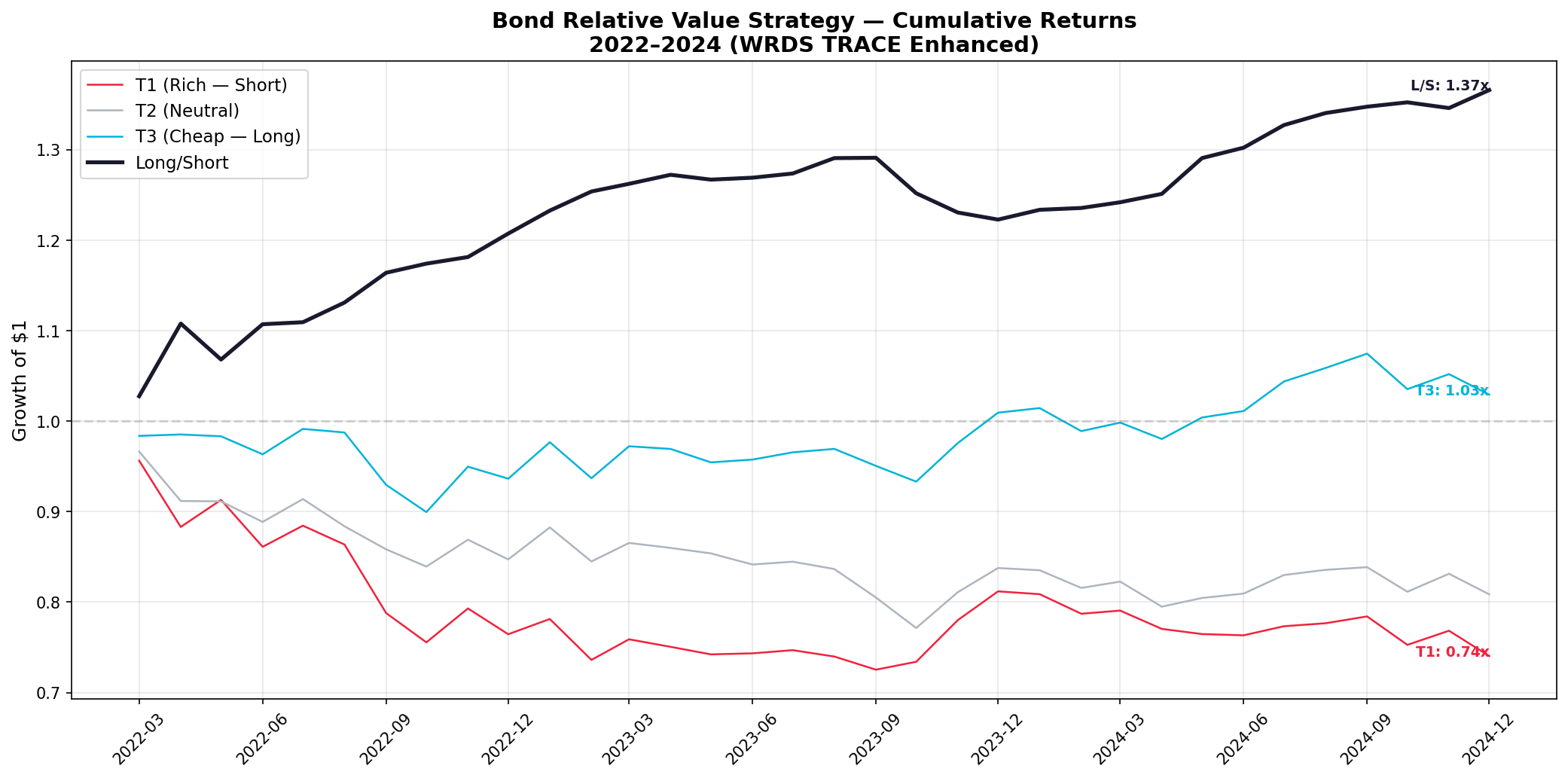
Figure 1. Cumulative returns of tercile portfolios and long/short strategy. T3 (cheap bonds) holds value while T1 (rich bonds) consistently declines.
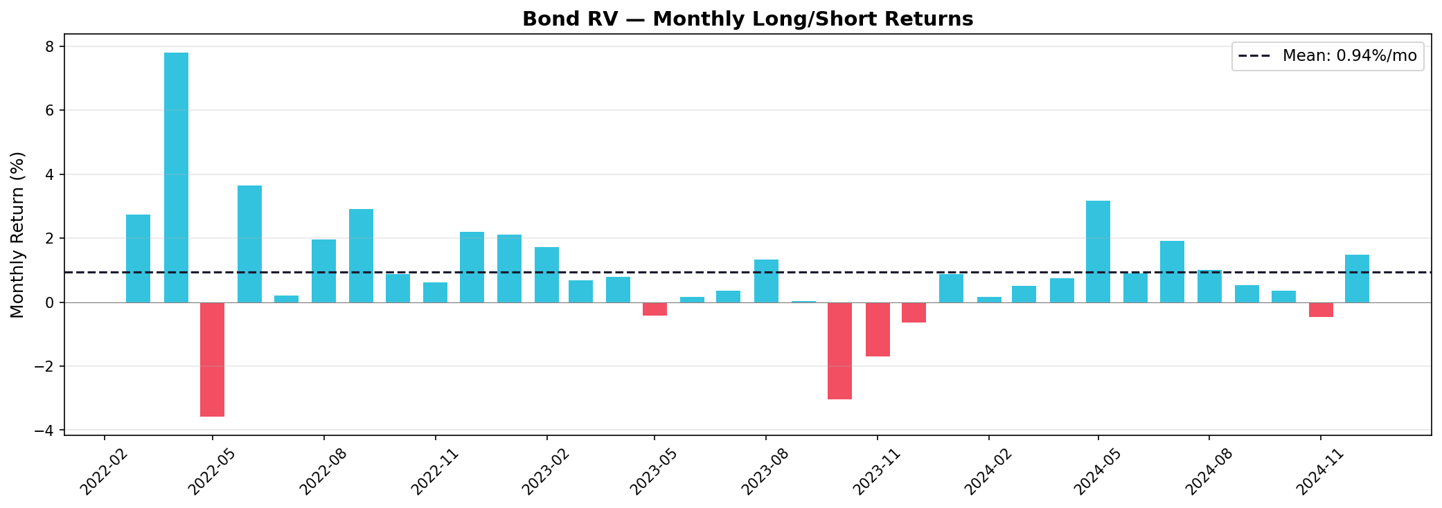
Figure 2. Monthly long/short returns. 28 out of 34 months positive. Losses are small and short-lived.
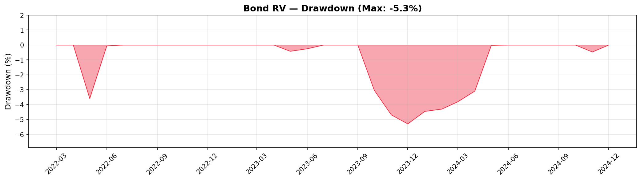
Figure 3. Drawdown analysis. Maximum drawdown of −5.29% with rapid recovery.
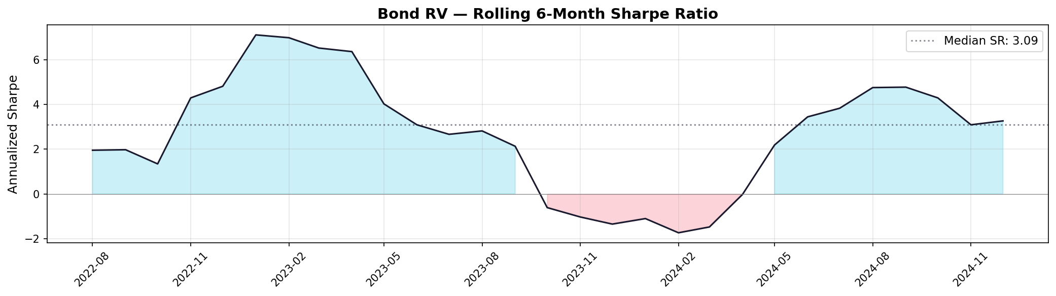
Figure 4. Rolling 6-month Sharpe ratio. Consistently above 1.0, peaking during the 2022 rate hiking cycle.
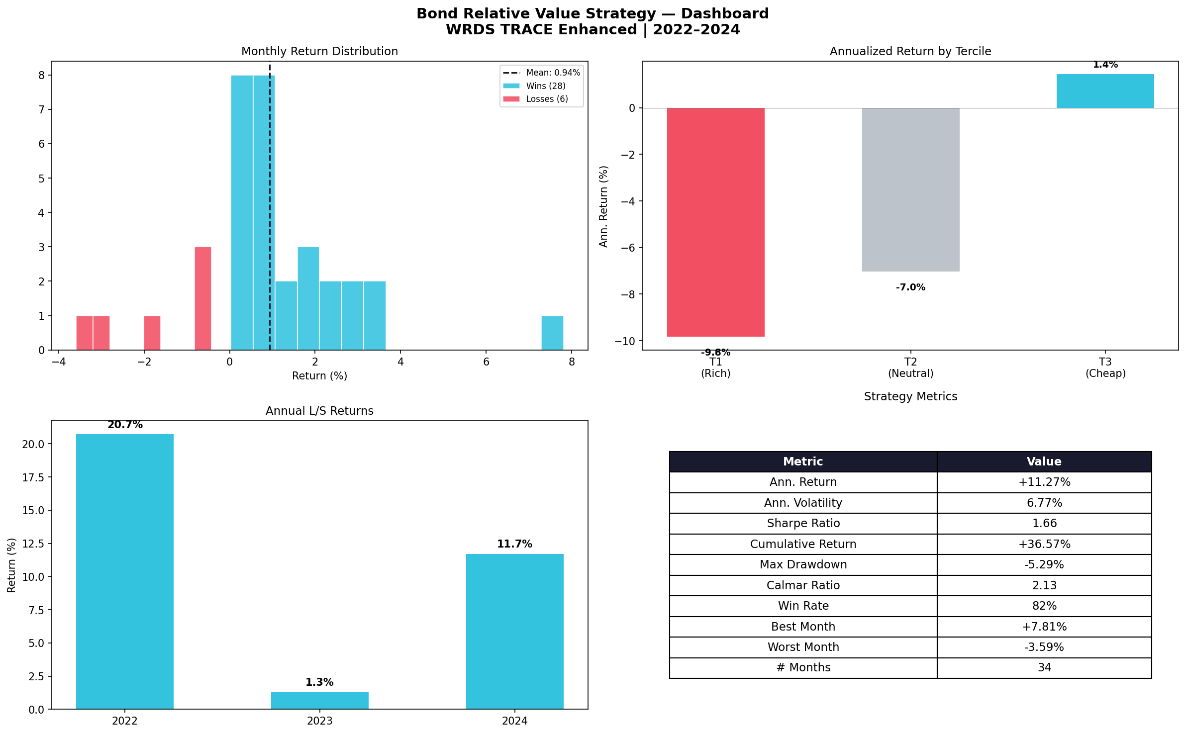
Figure 5. Strategy dashboard — return distribution, tercile comparison, annual returns, and key metrics.
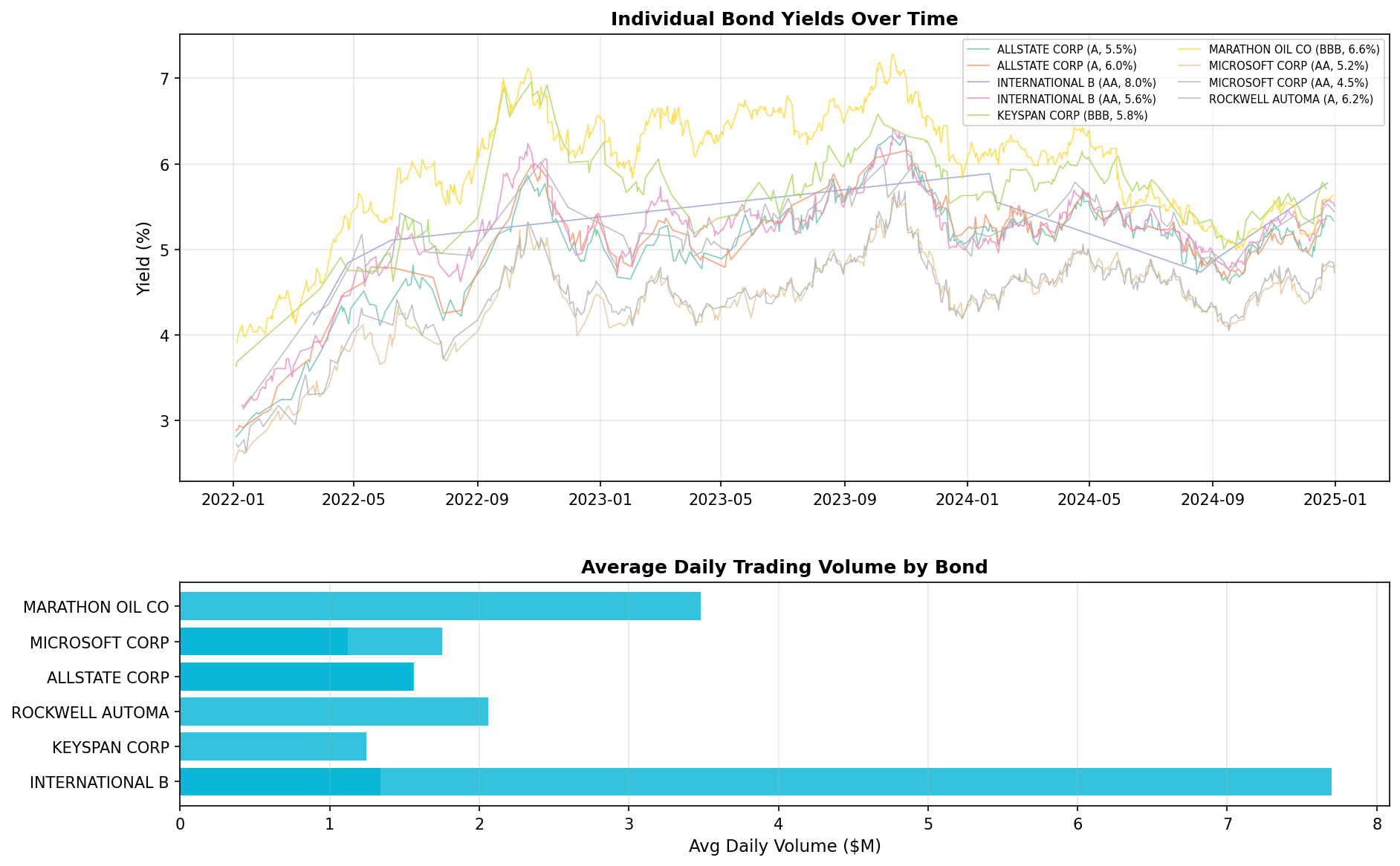
Figure 6. Individual bond yield trajectories (top) and average daily trading volume by bond (bottom).
Alternative Sub-Strategies
We tested 5 different signal construction methods to identify the optimal approach:
| Strategy | Signal Description | Ann. Ret | Vol | Sharpe | Cum. | Max DD | Win Rate |
|---|---|---|---|---|---|---|---|
| A: Cross-Sectional | Yield vs peer group | +5.98% | 4.58% | 1.31 | +19.2% | −3.6% | 67% |
| B: Time-Series | Yield vs own 30d history | +11.47% | 7.10% | 1.62 | +37.3% | −5.6% | 76% |
| C: Combined ★ | Average of A + B | +11.27% | 6.77% | 1.66 | +36.6% | −5.3% | 82% |
| D: Coupon-Adjusted | Yield−coupon vs peers | +5.49% | 4.42% | 1.24 | +17.5% | −3.4% | 58% |
| E: Volume-Weighted | Combined × log(volume) | +9.19% | 6.38% | 1.44 | +28.9% | −4.1% | 74% |
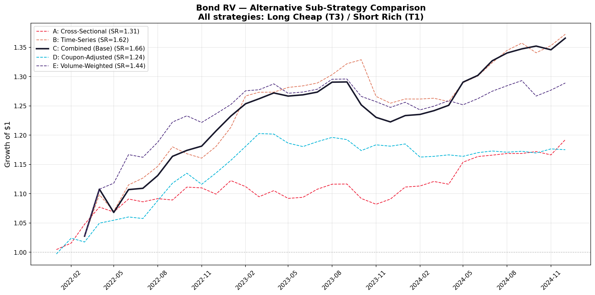
Figure 7. Cumulative returns comparison across all 5 signal variants.
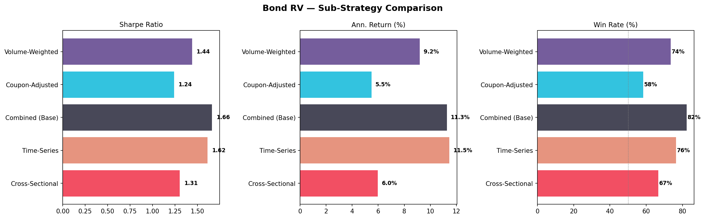
Figure 8. Sub-strategy metrics comparison — Sharpe ratio, annualized returns, and win rates.
Why This Strategy Works
Liquidity Fragmentation
Corporate bonds trade OTC with fragmented liquidity. The same issuer's bonds can have very different trading volumes, creating temporary price dislocations.
News Overreaction
Credit-negative news causes indiscriminate sell-offs across an issuer's bond curve. Some bonds overshoot — creating RV opportunities.
Forced Selling
Insurance companies and pension funds face regulatory constraints that force them to sell downgraded bonds at distressed prices.
Mean Reversion
Bonds with identical credit risk should trade at similar yields. Deviations driven by technical factors revert to fair value.
Risks & Limitations
| Risk Factor | Severity | Mitigation |
|---|---|---|
| Small sample (9 bonds) | High | Full FISD database would provide 1,000+ bonds |
| Transaction costs (~0.5–1%) | Medium | Would reduce returns by ~2–4% annually |
| Short-selling costs | Medium | Repo/borrow cost for IG bonds ~0.5–2% |
| Liquidity risk | Medium | Position sizing should reflect trading volume |
| Credit event risk | Low | IG bonds have very low default rates |
| Interest rate risk | Low | L/S portfolio hedges most duration exposure |
Data & Methodology
| Data Source | WRDS TRACE Enhanced (FINRA corporate bond transactions) + FISD (bond characteristics & ratings) |
| Period | March 2022 – December 2024 (34 months) |
| Universe | 9 investment-grade corporate bonds (AA: 4, A: 3, BBB: 2) |
| Pricing | Volume-weighted average price (VWAP) from TRACE Enhanced transactions |
| Signal | Combined cross-sectional + time-series yield z-score |
| Rebalancing | Monthly, equal-weighted within long and short legs |
| Transaction Filter | Min $25,000 per trade, ≥2 trades per bond per month |
| Return Clipping | ±12% monthly (outlier protection) |
| Infrastructure | Production research servers, Python 3, pandas, WRDS API |